Macro Dynamics with a Job Guarantee – Part 2: Keynesian Cross Diagram

by
peterc
My articles My booksMy videos
Follow on:Twitter

As a preliminary exercise, it may be instructive to modify the familiar Keynesian cross diagram to include the effects of a job guarantee within a simple short-run framework. The diagram includes two key schedules. The first is a 45-degree line showing all points for which actual expenditure equals actual income. The second is a line with lesser slope depicting the level of planned expenditure (total demand) at each level of income. Under appropriate conditions, the two schedules intersect at a steady-state level of income.

 
Simplifying assumptions

Some assumptions are made for simplicity. In particular, the following variables and parameters are taken as exogenously given:

1. The size of the labor force.
2. The total level of employment.
3. Within-sector productivity.
4. Total productive capacity.
5. The marginal propensity to leak to taxes, saving and imports.

Apart from 2, the assumptions are akin to those often employed in short-run macro models. Under these assumptions, variations in the economy’s total level of production require some workers to switch between higher-productivity sector b (the broader economy) and lower-productivity sector j (the job-guarantee program).

 
The demand function

In constructing the Keynesian cross diagram, the main task is to specify the characteristics of the demand schedule. In particular, the aim is to express total demand as a function of total income and graph the result, with total income represented along the horizontal axis and expenditure along the vertical axis. To this end, total demand will be considered the sum of three broad components: induced private consumption C_I, job-guarantee spending G_j and autonomous demand A.

Autonomous demand includes all exogenous spending on the economy’s output, whether by domestic households, firms and government or by foreigners, and is considered net of exogenous taxes and exogenous imports. Autonomous demand is not directly related to current income and, for the purposes of the model, is simply taken as given. Graphically, it is represented by a horizontal straight line with vertical intercept (0,A), indicating that this component of planned expenditure remains constant over all possible levels of income.

Induced private consumption refers to the part of domestic household consumption that is directly related to current income. Induced private consumption is taken to be net of endogenous taxes and endogenous imports. By assumption, a constant fraction of an increment in income is induced to private consumption. The remaining fraction – also constant – drains to taxes, saving and imports. Induced private consumption is therefore an increasing function of income:

Here, α is the marginal propensity to leak to taxes, saving and imports, with 0 < α < 1. This makes 1 – α the net marginal propensity to consume. With α assumed constant, induced private consumption is a linear function of total income Y which starts from the origin and has positive slope 1 – α.

Job-guarantee spending. Conceptualizing the government’s spending on the job guarantee in a way suitable for graphing takes a little more work. It is clear that job-guarantee spending will be some proportion of total income: G_j = jY. The complication in this expression is that both j and Y are endogenous variables. For the purposes of graphing, it will be helpful to express j as a function of Y so as to relate job-guarantee spending explicitly just to one endogenous variable.

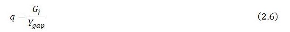
This can be done by considering job-guarantee spending from a different angle. While job-guarantee spending can be regarded as a proportion j of total income, it can equally be thought of as some fraction q of the output gap, where the output gap is defined to be the difference between maximum possible output and actual output:

Maximum possible output is the output that conceivably could be produced if all employment were located in sector b. This notional level of output depends only on sector b productivity (ρ_b) and total employment (L), both of which are assumed exogenous:

Substituting this expression for maximum output into (2.3) enables us to write job-guarantee spending as a function of total income:

Since sector b productivity and total employment are simply taken as given, the functional form of (2.5) will depend only on q. Job-guarantee spending will be a linear function of Y if q is a constant.

From rearrangement of (2.3),

If the quotient on the right-hand side is constant, q will also be constant.

The numerator of (2.6) is job-guarantee spending, which can be written

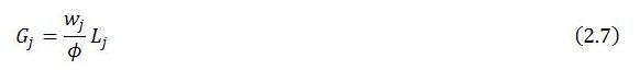
This is an identity. The fraction w_j/ϕ (the policy-administered job-guarantee wage divided by the wage share in job-guarantee spending) is the amount the government spends on the job guarantee per unit of sector j employment. The job-guarantee wage is taken as given on the basis that it will be set by policy. Less realistically, the wage share in job-guarantee spending is also taken as given, purely for simplicity. With w_j and ϕ both constant, w_j/ϕ is also a constant. Multiplying this fraction by sector j employment gives the level of job-guarantee spending.

The denominator of (2.6) is the output gap. This gap is created by the necessity, relating to the needs of price stability, for policymakers to maintain a degree of slack in the broader economy. This causes some employment to be located in sector j, where productivity (defined to be equal to w_j) is lower than in the broader economy (ρ_b). For every unit of employment located in sector j, there is forgone output of ρ_b – w_j. Accordingly,

Substituting the expressions for job-guarantee spending and the output gap given in (2.7) and (2.8) into the equation for q appearing in (2.6) gives

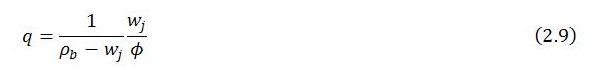
Under present assumptions all elements on the right-hand side of (2.9) are exogenously given, making q a constant. This, in turn, makes job-guarantee spending, as expressed in (2.5), a linear function of total income with vertical intercept (0,qρ_bL), horizontal intercept (ρ_bL,0) and negative slope -q. The negative slope represents the inverse relationship between job-guarantee spending and total income. The government’s spending on the job guarantee declines as income grows and rises when the economy contracts.

Total demand is simply the sum of its three broad components. Since all these components – induced private consumption, job-guarantee spending and autonomous demand – are linear functions of Y, so too is total demand.

The appropriate expression for total demand can be obtained by substituting the expressions for induced private consumption (2.2) and job-guarantee spending (2.5) into demand equation (2.1). Alternatively, the desired expression can be obtained by noting that

and substituting a suitable expression for j. Since j is defined as job-guarantee spending divided by total income, the desired equation can be found by dividing both sides of (2.5) by total income. This gives j as a function of Y:

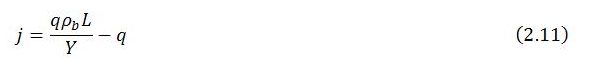
Upon substitution into (2.10):

This expression is a little more cumbersome than (2.10) but easy to understand and straightforward to graph. It shows total demand to be a straight line with vertical intercept (0,qρ_bL+A) and slope 1 – α – q.

Importantly, the demand function has lesser slope than the 45-degree line that is used in the Keynesian cross diagram to depict all points of equality between actual income and actual expenditure. Whereas the 45-degree line has a slope of 1, the demand function’s slope is less than 1 because α and q are always positive. This ensures that demand always crosses the 45-degree line at some level of output provided qρ_bL + A is positive.

Steady state. The point of intersection between the 45-degree line and the demand function can be found by substituting the right-hand side of (2.12) for demand in the equilibrium condition Y = Y_d and solving for Y. This gives the level of steady-state income:

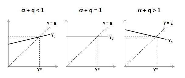
The inclusion of a job guarantee introduces a couple of points of difference with respect to the base model without a job guarantee. One difference is that even if autonomous demand were zero, the demand function’s vertical intercept would still be positive so long as total employment and sector b productivity were both positive because of the qρ_bL term in (2.12). Another difference is that the demand function need not necessarily be upward sloping but in principle can be upward sloping, horizontal or downward sloping depending on the values of α and q.

 
Graphing the model

With the demand function now specified it is straightforward to construct the Keynesian cross diagram. The first figure below shows the constituent parts of total demand as well as its overall level. The demand schedule intersects the 45-degree line at Y*, which is the steady-state level of income. In fact, under present assumptions, most notably that autonomous demand is constant rather than growing over time, the economy is stationary at income level Y*. The steady-state level of income only changes when there is a change in one of the parameters or exogenous variables.

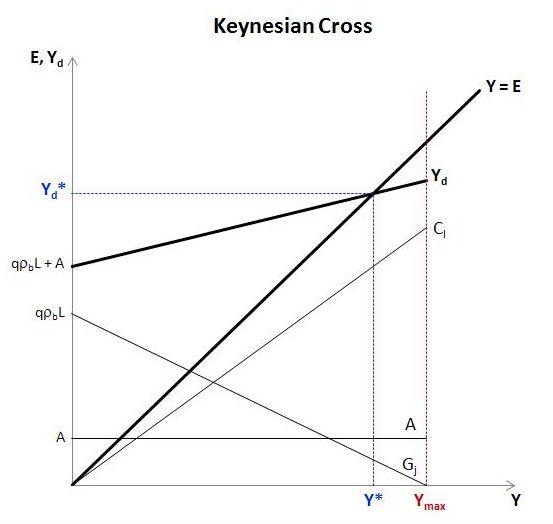
In the situation depicted, total demand is upward sloping. This will be the case whenever the sum of α and q is smaller than 1, since then the slope of the demand schedule (equal to 1 – α – q) is positive. More generally, the slope of the demand function can be positive, zero or negative, though it will always be less than 1, the slope of the 45-degree line.

The property that the demand function always has a slope less than one is critical to the system’s dynamic stability. It ensures that whenever the economy is at a level of output other than Y*, the tendency will be for the economy to return to the steady state.

In the Keynesian cross diagram, the area to the left and above the 45-degree line shows points of excess demand in which actual expenditure (E) exceeds the current level of production (Y). Conversely, the area to the right and below the 45-degree line shows points of excess supply. In the following diagram, the economy is at point (Y₀,Y_d0) with excess demand.

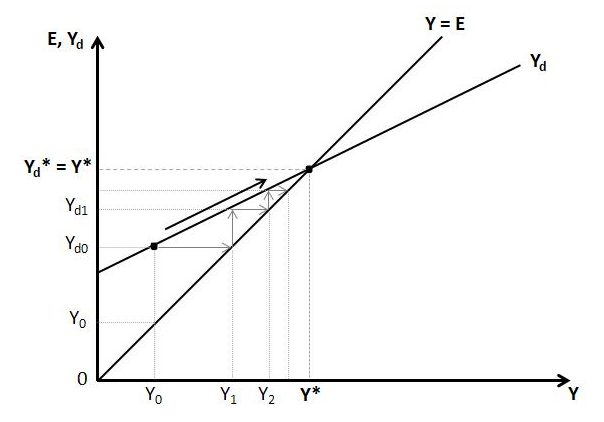
In the exaggerated scenario presented firms have produced output of Y₀. This falls short of demand Y_d0. In the initial instance, firms cater to the excess demand by running down inventories. They then interpret this unexpected depletion of inventories as a signal to expand production.

In general, it can be assumed that firms will alter the level of production by some proportion λ of the excess demand. For simplicity, the diagram is constructed on the assumption that λ = 1, which means that firms increase output in the next time step by the full amount of excess demand in the present time step. Accordingly, in the first time step output is expanded from Y₀ to Y₁.

This does not immediately restore the economy to the steady state because the expansion of output, by creating a higher flow of income, induces an additional change in demand. On the one hand, private consumption is positively affected; on the other, job-guarantee spending declines. In the particular scenario depicted, the demand schedule is upward sloping. This means that the boost to induced private consumption outweighs the impact on job-guarantee spending. The combined effect on demand is represented as a movement up along the demand schedule to the point (Y₁,Y_d1).

At output Y₁ there is once again some excess demand. However, there is less excess demand than previously because of the important property that the demand schedule has slope of less than 1. This, together with the assumption that qρ_bL + A is positive, is sufficient to engender (in the absence of exogenous shocks) a general tendency for the economy to tend toward the steady-state level of income Y*. Given time, in other words, output will catch up to demand.

The economic reason for the demand function’s slope being less than 1, which is the basis for any tendency toward a steady state, is that part of any additional income drains to taxes, saving and imports (the fraction α) and some job-guarantee spending is withdrawn (a fraction q) due to net migration of workers into the broader economy. This ensures that, when the economy is outside the steady state, the necessary variation in production and the change in demand it induces are smaller at each subsequent step of the adjustment process, with the effect that the impacts on output and demand get smaller and smaller, vanishing in the limit, as the steady state is approached.