Ergodicity — a questionable assumption (wonkish) .[embedded content] Paul Samuelson once famously claimed that the ‘ergodic hypothesis’ is essential for advancing economics from the realm of history to the realm of science. But is it really tenable to assume — as Samuelson and most other mainstream economists — that ergodicity is essential to economics? Sometimes ergodicity is mistaken for stationarity. But although all ergodic processes are stationary, they are not equivalent. Let’s say we have a stationary process. That does not guarantee that it is also ergodic. The long-run time average of a single output function of the stationary process may not converge to the expectation of the corresponding variables — and so the long-run time average may not
Topics:
Lars Pålsson Syll considers the following as important: Economics
This could be interesting, too:
Lars Pålsson Syll writes Schuldenbremse bye bye
Lars Pålsson Syll writes What’s wrong with economics — a primer
Lars Pålsson Syll writes Krigskeynesianismens återkomst
Lars Pålsson Syll writes Finding Eigenvalues and Eigenvectors (student stuff)
Ergodicity — a questionable assumption (wonkish)
.
Paul Samuelson once famously claimed that the ‘ergodic hypothesis’ is essential for advancing economics from the realm of history to the realm of science. But is it really tenable to assume — as Samuelson and most other mainstream economists — that ergodicity is essential to economics?
Sometimes ergodicity is mistaken for stationarity. But although all ergodic processes are stationary, they are not equivalent.
Let’s say we have a stationary process. That does not guarantee that it is also ergodic. The long-run time average of a single output function of the stationary process may not converge to the expectation of the corresponding variables — and so the long-run time average may not equal the probabilistic (expectational) average.
Say we have two coins, where coin A has a probability of 1/2 of coming up heads, and coin B has a probability of 1/4 of coming up heads. We pick either of these coins with a probability of 1/2 and then toss the chosen coin over and over again. Now let H1, H2, … be either one or zero as the coin comes up heads or tales. This process is obviously stationary, but the time averages — [H1 + … + Hn]/n — converges to 1/2 if coin A is chosen, and 1/4 if coin B is chosen. Both these time averages have a probability of 1/2 and so their expectational average is 1/2 x 1/2 + 1/2 x 1/4 = 3/8, which obviously is not equal to 1/2 or 1/4. The time averages depend on which coin you happen to choose, while the probabilistic (expectational) average is calculated for the whole “system” consisting of both coin A and coin B.
Instead of arbitrarily assuming that people have a certain type of utility function — as in mainstream theory — time average considerations show that we can obtain a less arbitrary and more accurate picture of real people’s decisions and actions by basically assuming that time is irreversible. When our assets are gone, they are gone. The fact that in a parallel universe, it could conceivably have been refilled, is of little comfort to those who live in the one and only possible world that we call the real world.
Time average considerations show that because we cannot go back in time, we should not take excessive risks. High leverage increases the risk of bankruptcy. This should also be a warning for the financial world, where the constant quest for greater and greater leverage — and risks — creates extensive and recurrent systemic crises.
Suppose I want to play a game. Let’s say we are tossing a coin. If heads come up, I win a dollar, and if tails come up, I lose a dollar. Suppose further that I believe I know that the coin is asymmetrical and that the probability of getting heads (p) is greater than 50% – say 60% (0.6) – while the bookmaker assumes that the coin is totally symmetric. How much of my bankroll (T) should I optimally invest in this game?
A strict mainstream utility-maximizing economist would suggest that my goal should be to maximize the expected value of my bankroll (wealth), and according to this view, I ought to bet my entire bankroll.
Does that sound rational? Most people would answer no to that question. The risk of losing is so high, that I already after a few games played — the expected time until my first loss arises is 1/(1-p), which in this case is equal to 2.5 — with a high likelihood would be losing and thereby become bankrupt. The expected-value maximizing economist does not seem to have a particularly attractive approach.
So what are the alternatives? One possibility is to apply the so-called Kelly criterion — after the American physicist and information theorist John L. Kelly, who in the article A New Interpretation of Information Rate (1956) suggested this criterion for how to optimize the size of the bet — under which the optimum is to invest a specific fraction (x) of wealth (T) in each game. How do we arrive at this fraction?
When I win, I have (1 + x) times as much as before, and when I lose (1 – x) times as much. After n rounds, when I have won v times and lost n – v times, my new bankroll (W) is
(1) W = (1 + x)v(1 – x)n – v T
(A technical note: The bets used in these calculations are of the “quotient form” (Q), where you typically keep your bet money until the game is over, and a fortiori, in the win/lose expression it’s not included that you get back what you bet when you win. If you prefer to think of odds calculations in the “decimal form” (D), where the bet money typically is considered lost when the game starts, you have to transform the calculations according to Q = D – 1.)
The bankroll increases multiplicatively — “compound interest” — and the long-term average growth rate for my wealth can then be easily calculated by taking the logarithms of (1), which gives
(2) log (W/ T) = v log (1 + x) + (n – v) log (1 – x).
If we divide both sides by n we get
(3) [log (W / T)] / n = [v log (1 + x) + (n – v) log (1 – x)] / n
The left-hand side now represents the average growth rate (g) in each game. On the right-hand side, the ratio v/n is equal to the percentage of bets that I won, and when n is large, this fraction will be close to p. Similarly, (n – v)/n is close to (1 – p). When the number of bets is large, the average growth rate is
(4) g = p log (1 + x) + (1 – p) log (1 – x).
Now we can easily determine the value of x that maximizes g:
(5) d [p log (1 + x) + (1 – p) log (1 – x)]/d x = p/(1 + x) – (1 – p)/(1 – x) =>
p/(1 + x) – (1 – p)/(1 – x) = 0 =>
(6) x = p – (1 – p)
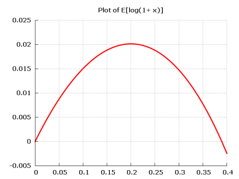
Since p is the probability that I will win, and (1 – p) is the probability that I will lose, the Kelly strategy says that to optimize the growth rate of your bankroll (wealth) you should invest a fraction of the bankroll equal to the difference of the likelihood that you will win or lose. In our example, this means that I have in each game to bet the fraction of x = 0.6 – (1 – 0.6) ≈ 0.2 — that is, 20% of my bankroll. Alternatively, we see that the Kelly criterion implies that we have to choose x so that E[log(1+x)] — which equals p log (1 + x) + (1 – p) log (1 – x) — is maximized. Plotting E[log(1+x)] as a function of x we see that the value maximizing the function is 0.2:
The optimal average growth rate becomes
(7) 0.6 log (1.2) + 0.4 log (0.8) ≈ 0.02.
If I bet 20% of my wealth in tossing the coin, I will after 10 games on average have 1.0210 times more than when I started (≈ 1.22).
This game strategy will give us an outcome in the long run that is better than if we use a strategy building on the mainstream theory of choice under uncertainty (risk) – expected value maximization. If we bet all our wealth in each game we will most likely lose our fortune, but because with low probability we will have a very large fortune, the expected value is still high. For a real-life player – for whom there is very little to benefit from this type of ensemble average – it is more relevant to look at the time average of what he may be expected to win (in our game the averages are the same only if we assume that the player has a logarithmic utility function). What good does it do me if my tossing the coin maximizes an expected value when I might have gone bankrupt after four games played? If I try to maximize the expected value, the probability of bankruptcy soon gets close to one. Better then to invest 20% of my wealth in each game and maximize my long-term average wealth growth!
When applied to the mainstream theory of expected utility, one thinks in terms of a “parallel universe” and asks what is the expected return of an investment, calculated as an average over the “parallel universe”? In our coin toss example, it is as if one supposes that various “I” are tossing a coin and that the loss of many of them will be offset by the huge profits one of these “I” does. But this ensemble average does not work for an individual, for whom a time average better reflects the experience made in the “non-parallel universe” in which we live.
The Kelly criterion gives a more realistic answer, where one thinks in terms of the only universe we actually live in, and asks what the expected return of an investment — calculated as an average over time — is.
Since we cannot go back in time — entropy and the “arrow of time ” make this impossible — and the bankruptcy option is always at hand (extreme events and “black swans” are always possible) we have nothing to gain from thinking in terms of ensembles and “parallel universe.”
Actual events follow a fixed pattern of time, where events are often linked in a multiplicative process (e.g. investment returns with “compound interest”) which is basically non-ergodic.
Instead of arbitrarily assuming that people have a certain type of utility function – as in mainstream theory – the Kelly criterion shows that we can obtain a less arbitrary and more accurate picture of real people’s decisions and actions by basically assuming that time is irreversible. When the bankroll is gone, it’s gone. The fact that in a parallel universe, it could conceivably have been refilled, is of little comfort to those who live in the one and only possible world that we call the real world.
Our coin toss example can be applied to more traditional economic issues. If we think of an investor, we can basically describe his situation in terms of our coin toss. What fraction (x) of his assets (T) should an investor – who is about to make a large number of repeated investments – bet on his feeling that he can better evaluate an investment (p = 0.6) than the market (p = 0.5)? The greater the x, the greater the leverage. But also – the greater is the risk. Since p is the probability that his investment valuation is correct and (1 – p) is the probability that the market’s valuation is correct, it means the Kelly criterion says he optimizes the rate of growth on his investments by investing a fraction of his assets that is equal to the difference in the probability that he will “win” or “lose.” In our example this means that he at each investment opportunity is to invest the fraction of x = 0.6 – (1 – 0.6), i.e. about 20% of his assets. The optimal average growth rate of investment is then about 2 % (0.6 log (1.2) + 0.4 log (0.8)).
Kelly’s criterion shows that because we cannot go back in time, we should not take excessive risks. High leverage increases the risk of bankruptcy. This should also be a warning for the financial world, where the constant quest for greater and greater leverage — and risks – creates extensive and recurrent systemic crises. A more appropriate level of risk-taking is a necessary ingredient in a policy to curb excessive risk-taking.
The works of people like Ollie Hulme and Ole Peters at London Mathematical Laboratory show that expected utility theory is transmogrifying truth. Economics needs something different than a theory relying on arbitrary utility functions.
Added 1: If you know some Python, here’s a code you can run to plot and show the difference between a time average and an ensemble average:
import numpy as np

np.random.seed(0)

num_measurements = 200

num_samples = 20

measurements = np.random.randn(num_measurements, num_samples)

time_average = np.mean(measurements, axis=0)

ensemble_average = np.mean(measurements, axis=1)

import matplotlib.pyplot as plt

plt.figure(figsize=(10, 5))

plt.subplot(1, 2, 1)

plt.plot(time_average, range(num_samples), marker='o')

plt.title('Time Average')

plt.xlabel('Average Value')

plt.ylabel('Ensemble')

plt.grid(True)

plt.subplot(1, 2, 2)

plt.plot(range(num_measurements), ensemble_average, marker='o')

plt.title('Ensemble Average')

plt.xlabel('Measurement')

plt.ylabel('Average Value')

plt.grid(True)

plt.tight_layout()

plt.show()

Added 2: And if you're still not convinced it is a bad idea
to always treat things as if they were ergodic, maybe you
should try some Russian Roulette ...
import numpy as np
import matplotlib.pyplot as plt
def play_russian_roulette():
"""
Simulate playing Russian roulette.
Returns:
payoff: The payoff for the game (1000 if survives, 0 otherwise).
"""
if np.random.rand() < 1/6:
return 0
else:
return 1000
def expected_return(n):
"""
Calculate the expected return for a person playing Russian roulette for n rounds.
Args:
n: Number of rounds.
Returns:
exp_return: Expected return.
"""
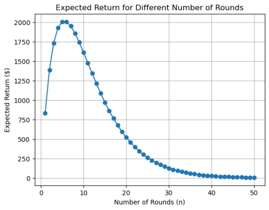
return (5/6)**n * 1000 * n
def plot_expected_return(max_rounds):
"""
Plot the expected return for each round.
Args:
max_rounds: Maximum number of rounds.
"""
expected_returns = [expected_return(n) for n in range(1, max_rounds + 1)]
plt.plot(range(1, max_rounds + 1), expected_returns, marker='o')
plt.title("Expected Return for Different Number of Rounds")
plt.xlabel("Number of Rounds (n)")
plt.ylabel("Expected Return ($)")
plt.grid(True)
plt.show()
if __name__ == "__main__":
max_rounds = 50
plot_expected_return(max_rounds)
As you will notice the expected return is not very promising ...