The job guarantee as proposed by Modern Monetary Theorists would provide a publicly funded job with defined wage and benefits to anyone who desired one, with public spending on the program varying automatically and countercyclically in response to take-up of positions. In a downturn, workers who lost their jobs would have the option of accepting the job-guarantee offer. As the economy recovered, some workers would receive better offers elsewhere. By design, the job-guarantee provider would not compete on wages in an attempt to retain such workers. Rather, the program would provide a stable wage floor, serving as a nominal price anchor for the economy. Periodically it would be appropriate to revise the program wage, but these wage adjustments would reflect factors such as trend
Topics:
peterc considers the following as important: Job & Income Guarantee
This could be interesting, too:
peterc writes Macro Dynamics with a Job Guarantee – Part 6: Price Stabilization
peterc writes Macro Dynamics with a Job Guarantee – Part 5: Price Level
peterc writes Macro Dynamics with a Job Guarantee – Part 4: Dynamic Stability
peterc writes Macro Dynamics with a Job Guarantee – Part 3: Adjustment Process
The job guarantee as proposed by Modern Monetary Theorists would provide a publicly funded job with defined wage and benefits to anyone who desired one, with public spending on the program varying automatically and countercyclically in response to take-up of positions. In a downturn, workers who lost their jobs would have the option of accepting the job-guarantee offer. As the economy recovered, some workers would receive better offers elsewhere. By design, the job-guarantee provider would not compete on wages in an attempt to retain such workers. Rather, the program would provide a stable wage floor, serving as a nominal price anchor for the economy. Periodically it would be appropriate to revise the program wage, but these wage adjustments would reflect factors such as trend improvements in the economy’s average productivity or distributional considerations rather than fluctuations in demand.
Earlier posts have considered various macro aspects of a job guarantee using a model developed within the familiar income-expenditure framework. The present post is the first in what may turn into an open-ended series attempting a more systematic treatment of the topic. The basic model is very simple but amenable to extension.
Broad overview
The model divides the economy into two broad sectors, the ‘broader economy’ or sector b and the ‘job-guarantee sector’ or sector j. Sector b covers all economic activity other than production undertaken specifically by job-guarantee workers. It includes as sub-sectors the domestic private sector, the external sector and all parts of the domestic public sector that are not directly engaged in job-guarantee employment. It is supposed that plant, equipment and materials used by sector j are supplied by the broader economy. Similarly, public administration of the job guarantee is regarded as activity of the broader economy.
The government’s spending on the job guarantee (Gj) is a variable proportion of total income (and output) Y such that Gj = jY. A fraction ϕ of this spending is on the wages of job-guarantee workers while the remaining fraction 1 – ϕ is on plant, equipment, materials and public administration of the program. Sector j output is evaluated as the wages paid to job-guarantee workers: Yj = ϕGj = ϕjY. All other income is generated by the broader economy: Yb = (1 – ϕj)Y. This makes the sectoral income shares ϕj and 1 – ϕj, which vary whenever j varies. For simplicity, ϕ is taken to be constant.
The model can be adapted to both short-run and long-run contexts.
At its simplest, the model applies to a short run in which productive capacity is taken as given and the economy is stationary other than when adjusting to one-off exogenous changes in demand. In this simplest form of the model, total employment and sector b productivity are taken as given. All demand other than induced net private consumption and job-guarantee spending are considered autonomous of income. Induced private consumption is assumed to vary directly with income in accordance with a constant net marginal propensity to consume, in contrast to the inverse (and variable) response of job-guarantee spending to changes in income.
In long run applications of the model, the economy (including its productive capacity) grows over time and private investment is considered endogenous, with the share of private investment in total income fluctuating procyclically at a variable rate. Both output and capacity are considered demand determined.
Irrespective of the time frame, the model allows a theoretical consideration of various demand effects on the level and composition of output as well as on the price level. Initially the focus will be on the behavior of output. Later, a way to represent the price-stabilizing aspect of a job guarantee can be introduced.
In considering the impact of an exogenous shock, three aspects of the economy’s adjustment process can be identified. First, for given values of the model’s parameters and exogenous variables, there is a steady state to which all the endogenous quantities and growth rates tend. Second, at any time during the adjustment from one steady state to another, there is a notional equilibrium at which total supply would equal total demand. These notional (moving) equilibria differ from the steady state and only coincide with it (other than incidentally) once a steady state is reached. Third, the actual adjustment of endogenous quantities and growth rates is distinct from the behavior of the moving equilibria. Actual quantities and growth rates only coincide (other than incidentally) with their steady state and equilibrium counterparts in a steady state. The relevance of steady states is that, within the model, they act as attractors for the actual levels and growth rates of the endogenous variables.
Basic framework
By way of introduction, and to illustrate the distinction between steady-state, equilibrium and actual adjustment processes, it is convenient to take a first glimpse at the model. The points about to be considered can be explored in more detail later but for now a broad overview will suffice. Consider an economy that is stationary other than when responding to an exogenous change in demand. Let A denote autonomous demand, α the marginal propensity to leak to taxes, saving and imports, and j the share of job-guarantee spending in total income Y. Induced consumption, net of endogenous imports, is (1 – α)Y, while job-guarantee spending is jY. The sum of these two spending components constitutes induced demand (1 – α + j)Y. The equilibrium condition and level of demand (Yd) are
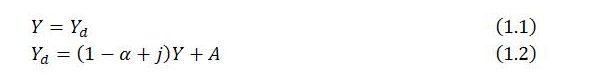
In the present context, output Y denotes the level of production, which can differ from sales. It is supposed that whenever the sum of planned expenditures (demand) differs from output (supply), the difference is met through unanticipated changes in inventories. In response to these unexpected movements in inventories, firms are assumed to alter production levels over time in an attempt to adjust output to demand. The level of output Ye that would correspond to an equilibrium situation is found by substituting the demand function into the equilibrium condition and solving for Y. This gives:
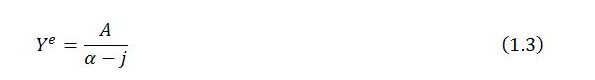
Autonomous demand (A) and the marginal propensity to leak (α) are both assumed to be constant. In contrast, the share of job-guarantee spending in income (j) is a variable and moves counter to the business cycle. The value of j at any time will imply, together with the constant values of A and α, a notional level of income (Ye) for which supply (Y) would equal demand (Yd). As (1.3) makes clear, this equilibrium level of income will change with every variation in j as the latter continually responds to the need for automatic adjustments in the sectoral composition of employment to keep the economy at full employment.
The equilibrium level of income is only consistent with a steady state once j stabilizes at its steady-state value j*. This only occurs if the sectoral composition of employment stabilizes. The steady-state level of income is
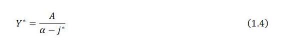
In a stationary economy, all terms in (1.4) are constant, including j*. So, in the simplest version of the model, a steady state is also a stationary state.
The value of j* can be known as soon as the values of the exogenous variables and parameters are chosen. The actual value of j, however, will depend on the process of economic adjustment. Within the model, the adjustment process is driven by sector b, which is assumed to react to disequilibrium in a particular way:
 Here, Yb‘ is the derivative of Yb with respect to time, Ydb and Yb are respectively the demand and output of sector b, and λ is a positive constant measuring the strength of the response of sector b to excess demand or excess supply (Ydb – Yb). As indicated by (1.5), variations in the output of sector b can also be related to excess demand for the economy as a whole (Yd – Y), rather than just to the excess demand of the sector itself, because of the nature of the job guarantee. By definition, sector j is always in equilibrium, with its income always equal to demand (Yj = Ydj). This is because sector j output (evaluated as the wages of job-guarantee workers) is synonymous with spending on the sector (government spending on job-guarantee wages). Since sector j is always in equilibrium, excess demand for the economy as a whole is always the same as excess demand in sector b (that is, Yd – Y = Ydb – Yb).
Substituting the expression for Yd in (1.2) into the reaction function for Yb in (1.5) and rearranging gives:

A steady state occurs when Yb‘ = 0. This requires
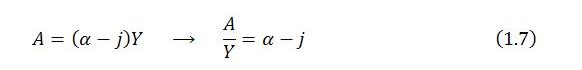
This says that the share of autonomous demand in total income (A/Y) must equal the net marginal propensity to leak (α – j) for the economy to be in a steady state. This condition can be compared with the expression for equilibrium income given in (1.3). Simple rearrangement of that expression shows that in equilibrium,
Unlike (1.7), the relation (1.8) holds at any time. It holds whether the system is in equilibrium or disequilibrium, and it holds whether the system is in or out of a steady state. It simply means that there is always a notional level of output at which the share of autonomous demand in total income would equal α – j. But a steady state requires that the actual share of autonomous demand in total income (A/Y) coincides with the equilibrium share (A/Ye). In a steady state,

This occurs when the share of job-guarantee spending in income has stabilized at its steady-state value (j = j*) such that:

The significance of the ratio A/Y for the behavior of the broader economy can be made explicit in the reaction function (1.6). Let z = A/Y, ze = A/Ye and z* = A/Y*. Sector b’s reaction function can then be written

Starting from a steady state, with z = ze = z*, a one-off exogenous change in demand dislodges z and Y from equilibrium and dislodges z, ze and Y from the steady state. The steady state itself instantly shifts to a new position that depends only on the values of the parameters and exogenous variables. Sector b reacts to the excess demand or supply in accordance with (1.11). This alters the level and composition of output and employment, with some workers switching sectors. In response, the share of job-guarantee spending in total income (j) continually adjusts, altering z and ze in the process. Once j reaches its new steady state, both z and ze stabilize at the new z*. At this point, Yb‘ is zero and there is no tendency for change in the absence of another exogenous shock to the system.
A look ahead
The foregoing is just a sketch of the conceptual framework. The framework permits the posing of standard theoretical questions in relation to a demand-led economy with a job guarantee, including:
- the properties of a steady state;
- system behavior outside the steady state in terms of both levels and growth rates as well as aggregates and sectoral composition;
- conditions for convergence to a steady state (dynamic stability); and
- stabilizing effects of a job guarantee on output, employment and the price level.
While the presentation will initially be kept as simple as possible, with attention confined to a short run in which productive capacity is fixed, the model can be extended to consider a continually growing economy in which
- private investment is endogenous;
- output and capacity are both demand determined;
- the size of the labor force and total employment vary; and
- productivity of the broader economy is endogenous.
For now, though, introducing these features would complicate matters without adding much of significance on the points to be considered.
Academic material
There is an extensive academic literature on the job guarantee. The theoretical underpinnings of the policy proposal are set out in:
Bill Mitchell – The Buffer Stock Employment Model and the NAIRU: The Path to Full Employment
Warren Mosler – Full Employment AND Price Stability
Scholarly analyses of the stabilizing properties of a job guarantee include:
Scott Fullwiler – Macroeconomic Stabilization Through an Employer of Last Resort
Warren Mosler and Damiano Silipo – Maximizing Price Stability in a Monetary Economy
Related heteconomist posts
A number of earlier posts are closely related to the present one. Of these, some focus on macro effects of a job guarantee:
Job Guarantee as Nominal Price Anchor
The Income-Expenditure Model with a Job Guarantee
Some Macro Effects of a Job Guarantee
Quantity Dynamics with a Job Guarantee
Some Aspects of a Steady State with a Job Guarantee
Illustration of Dynamic Adjustment with a Job Guarantee
Other posts relate to the basic theoretical framework:
Condensed Income-Expenditure Model
A Notion of Demand-Led Growth
A Simple Framework for Analyzing a Demand-Led Economy
Disequilibrium Dynamics of Output and Demand
Dynamics of Output and Demand in a Growing Economy