Expected utility theory — a severe case of transmogrifying truth Although the expected utility theory is obviously both theoretically and descriptively inadequate, colleagues and microeconomics textbook writers all over the world gladly continue to use it, as though its deficiencies were unknown or unheard of. Daniel Kahneman writes — in Thinking, Fast and Slow — that expected utility theory is seriously flawed since it doesn’t take into consideration the basic fact that people’s choices are influenced by changes in their wealth. Where standard microeconomic theory assumes that preferences are stable over time, Kahneman and other behavioural economists have forcefully again and again shown that preferences aren’t fixed, but vary with different reference
Topics:
Lars Pålsson Syll considers the following as important: Economics
This could be interesting, too:
Lars Pålsson Syll writes Schuldenbremse bye bye
Lars Pålsson Syll writes What’s wrong with economics — a primer
Lars Pålsson Syll writes Krigskeynesianismens återkomst
Lars Pålsson Syll writes Finding Eigenvalues and Eigenvectors (student stuff)
Expected utility theory — a severe case of transmogrifying truth
Although the expected utility theory is obviously both theoretically and descriptively inadequate, colleagues and microeconomics textbook writers all over the world gladly continue to use it, as though its deficiencies were unknown or unheard of.
Daniel Kahneman writes — in Thinking, Fast and Slow — that expected utility theory is seriously flawed since it doesn’t take into consideration the basic fact that people’s choices are influenced by changes in their wealth. Where standard microeconomic theory assumes that preferences are stable over time, Kahneman and other behavioural economists have forcefully again and again shown that preferences aren’t fixed, but vary with different reference points. How can a theory that doesn’t allow for people having different reference points from which they consider their options have an almost axiomatic status within economic theory?
The mystery is how a conception of the utility of outcomes that is vulnerable to such obvious counterexamples survived for so long. I can explain it only by a weakness of the scholarly mind … I call it theory-induced blindness: once you have accepted a theory and used it as a tool in your thinking it is extraordinarily difficult to notice its flaws … You give the theory the benefit of the doubt, trusting the community of experts who have accepted it … But they did not pursue the idea to the point of saying, “This theory is seriously wrong because it ignores the fact that utility depends on the history of one’s wealth, not only present wealth.”

On a more economic-theoretical level, information theory — and especially the so-called Kelly criterion — also highlights the problems concerning the neoclassical theory of expected utility. Suppose I want to play a game. Let’s say we are tossing a coin. If heads come up, I win a dollar, and if tails come up, I lose a dollar. Suppose further that I believe I know that the coin is asymmetrical and that the probability of getting heads (p) is greater than 50% – say 60% (0.6) – while the bookmaker assumes that the coin is totally symmetric. How much of my bankroll (T) should I optimally invest in this game?
A strict neoclassical utility-maximizing economist would suggest that my goal should be to maximize the expected value of my bankroll (wealth), and according to this view, I ought to bet my entire bankroll.
Does that sound rational? Most people would answer no to that question. The risk of losing is so high, that I already after few games played — the expected time until my first loss arises is 1/(1-p), which in this case is equal to 2.5 — with a high likelihood would be losing and thereby become bankrupt. The expected-value maximizing economist does not seem to have a particularly attractive approach.
 So what’s the alternative? One possibility is to apply the so-called Kelly criterion — after the American physicist and information theorist John L. Kelly, who in the article A New Interpretation of Information Rate (1956) suggested this criterion for how to optimize the size of the bet — under which the optimum is to invest a specific fraction (x) of wealth (T) in each game. How do we arrive at this fraction?
When I win, I have (1 + x) times as much as before, and when I lose (1 – x) times as much. After n rounds, when I have won v times and lost n – v times, my new bankroll (W) is
(1) W = (1 + x)v(1 – x)n – v T
[A technical note: The bets used in these calculations are of the “quotient form” (Q), where you typically keep your bet money until the game is over, and a fortiori, in the win/lose expression it’s not included that you get back what you bet when you win. If you prefer to think of odds calculations in the “decimal form” (D), where the bet money typically is considered lost when the game starts, you have to transform the calculations according to Q = D – 1.]
The bankroll increases multiplicatively — “compound interest” — and the long-term average growth rate for my wealth can then be easily calculated by taking the logarithms of (1), which gives
(2) log (W/ T) = v log (1 + x) + (n – v) log (1 – x).
If we divide both sides by n we get
(3) [log (W / T)] / n = [v log (1 + x) + (n – v) log (1 – x)] / n
The left-hand side now represents the average growth rate (g) in each game. On the right-hand side the ratio v/n is equal to the percentage of bets that I won, and when n is large, this fraction will be close to p. Similarly, (n – v)/n is close to (1 – p). When the number of bets is large, the average growth rate is
(4) g = p log (1 + x) + (1 – p) log (1 – x).
Now we can easily determine the value of x that maximizes g:
(5) d [p log (1 + x) + (1 – p) log (1 – x)]/d x = p/(1 + x) – (1 – p)/(1 – x) =>
p/(1 + x) – (1 – p)/(1 – x) = 0 =>
(6) x = p – (1 – p)
Since p is the probability that I will win, and (1 – p) is the probability that I will lose, the Kelly strategy says that to optimize the growth rate of your bankroll (wealth) you should invest a fraction of the bankroll equal to the difference of the likelihood that you will win or lose. In our example, this means that I have in each game to bet the fraction of x = 0.6 – (1 – 0.6) ≈ 0.2 — that is, 20% of my bankroll. Alternatively, we see that the Kelly criterion implies that we have to choose x so that E[log(1+x)] — which equals p log (1 + x) + (1 – p) log (1 – x) — is maximized. Plotting E[log(1+x)] as a function of x we see that the value maximizing the function is 0.2:
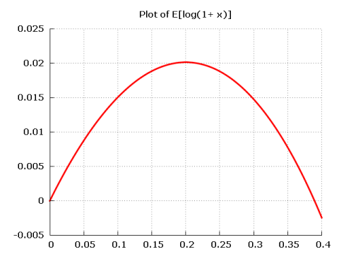
The optimal average growth rate becomes
(7) 0.6 log (1.2) + 0.4 log (0.8) ≈ 0.02.
If I bet 20% of my wealth in tossing the coin, I will after 10 games on average have 1.0210 times more than when I started (≈ 1.22).
This game strategy will give us an outcome in the long run that is better than if we use a strategy building on the neoclassical economic theory of choice under uncertainty (risk) – expected value maximization. If we bet all our wealth in each game we will most likely lose our fortune, but because with low probability we will have a very large fortune, the expected value is still high. For a real-life player – for whom there is very little to benefit from this type of ensemble-average – it is more relevant to look at time-average of what he may be expected to win (in our game the averages are the same only if we assume that the player has a logarithmic utility function). What good does it do me if my tossing the coin maximizes an expected value when I might have gone bankrupt after four games played? If I try to maximize the expected value, the probability of bankruptcy soon gets close to one. Better then to invest 20% of my wealth in each game and maximize my long-term average wealth growth!
When applied to the neoclassical theory of expected utility, one thinks in terms of a “parallel universe” and asks what is the expected return of an investment, calculated as an average over the “parallel universe”? In our coin toss example, it is as if one supposes that various “I” are tossing a coin and that the loss of many of them will be offset by the huge profits one of these “I” does. But this ensemble-average does not work for an individual, for whom a time-average better reflects the experience made in the “non-parallel universe” in which we live.
The Kelly criterion gives a more realistic answer, where one thinks in terms of the only universe we actually live in and ask what is the expected return of an investment, calculated as an average over time.
Since we cannot go back in time — entropy and the “arrow of time ” make this impossible — and the bankruptcy option is always at hand (extreme events and “black swans” are always possible) we have nothing to gain from thinking in terms of ensembles and “parallel universe.”
Actual events follow a fixed pattern of time, where events are often linked in a multiplicative process (as e. g. investment returns with “compound interest”) which is basically non-ergodic.
Instead of arbitrarily assuming that people have a certain type of utility function – as in the neoclassical theory – the Kelly criterion shows that we can obtain a less arbitrary and more accurate picture of real people’s decisions and actions by basically assuming that time is irreversible. When the bankroll is gone, it’s gone. The fact that in a parallel universe it could conceivably have been refilled, is of little comfort to those who live in the one and only possible world that we call the real world.
Our coin toss example can be applied to more traditional economic issues. If we think of an investor, we can basically describe his situation in terms of our coin toss. What fraction (x) of his assets (T) should an investor – who is about to make a large number of repeated investments – bet on his feeling that he can better evaluate an investment (p = 0.6) than the market (p = 0.5)? The greater the x, the greater is the leverage. But also – the greater is the risk. Since p is the probability that his investment valuation is correct and (1 – p) is the probability that the market’s valuation is correct, it means the Kelly criterion says he optimizes the rate of growth on his investments by investing a fraction of his assets that is equal to the difference in the probability that he will “win” or “lose.” In our example, this means that he at each investment opportunity is to invest the fraction of x = 0.6 – (1 – 0.6), i.e. about 20% of his assets. The optimal average growth rate of investment is then about 2 % (0.6 log (1.2) + 0.4 log (0.8)).
Kelly’s criterion shows that because we cannot go back in time, we should not take excessive risks. High leverage increases the risk of bankruptcy. This should also be a warning for the financial world, where the constant quest for greater and greater leverage – and risks – creates extensive and recurrent systemic crises. A more appropriate level of risk-taking is a necessary ingredient in a policy to come to curb excessive risk-taking.
The works of people like Kelly and Kahneman show that expected utility theory is indeed transmogrifying truth.